Enterprise Storage Synthetic Benchmarking Guide and Best Practices. Part 3. Practical Illustration based on Benchmarking VMware vSAN Case.

Well, let's go through the points outlined in Part 1 and Part 2 and look at an example of how testing might look end-to-end.

As I said, it is always worth starting with defining the goals and objectives. The true purpose of further benchmarks is to demonstrate with the specific example the process of conducting tests, as well as to illustrate the influence of individual parameters on test’s results. To make it closer to reality, let's come up with some kind of hypothetical, but still realistic situation.

Scenario and definition of objectives.

For starters, let’s imagine a company that built a VMware-based private cloud infrastructure some time ago. But it is used exclusively for software development and testing tasks, and even then, it provides only a partial coverage. The rest of the services run on a conventional VMware vSphere virtualization platform outside of the private cloud. Private cloud infrastructure, as well as the production environment, was built according to the traditional 3-tier architecture with blade servers, FC-network, SAN storage arrays and external hardware-defined network and security solutions.

It's been in use like this for quite a while, but, at some point in time, business stakeholders started to push for more speed and flexibility on the IT side. Responding to business needs, several strategic decisions were made:

• Cloud-first approach. All and every resource should be provisioned from the cloud management platform.
• Enable hybrid-cloud. Apps will be deployed both in the VMware-based private cloud infrastructure and in public clouds.
• Self-governance. Application owners can choose where to provision their workloads, factoring in compliance, security, cost, availability, and other requirements.

At the same time, there was a need to refresh the private cloud infrastructure under, as it was already deprecated, and no longer met the requirements. When developing the new platform’s architecture, the following key requirements were identified:

• Flexible and fast scaling that can be done in small steps. This is important because it is difficult to predict where developers will deploy their applications and how many, so infrastructure must be able to adapt fast. 
• Cost efficiency. Onprem infrastructure must offer competitive resource costs when compared to public clouds.
• Significant simplification of infrastructure operation, as many IT specialists will be reassigned to create a set of new high-value easy-to-consume onprem services similar to those available in the public clouds.

To meet those requirements, VMware hyper-converged infrastructure was considered as the primary option for the next generation of private cloud infrastructure. The next task was to draft a design and size clusters running the new private cloud, including the underlying hardware. With that in mind, the existing infrastructure was analyzed to obtain the averaged ratio of VMs’ vCPU/vRAM/Disk. That allows to make a coarse dimensioning for the new cluster. But storage performance assessment absolutely required confirmation and refinements.

So, the benchmark goals were defined as follows:

• Determine how many “averaged” VMs could be deployed on the cluster from the storage performance perspective to assess an averaged VM’s TCO for the new private cloud and to achieve a better hardware utilization.
• Understand the cluster's performance potential.
• Admins need to learn the specifics of the hyper converged platform, its behavior in different situations and under different loads, as well as potential bottlenecks.

Synthetic tests were chosen as a testing method because the workloads are expected to be very diverse, there are no workloads identified as particularly critical to be assessed individually, and, moreover, most workloads do not exist yet. The second reason is related to the fact that the use of synthetic benchmarks allows for the most flexible testing process and storage system’s behavior understanding.

It was decided to leverage HCIBench for the tests. The first reason for this was because the new private cloud platform will be built with VMware solutions. Another reason was that the test program included a large number of more or less standard tests that HCIBench fitted very well with.

Once we have decided on the benchmarking goals and methods, we need to collect some key metrics allowing us to define the success criteria. First, we need to understand from which segment of the infrastructure we can get them and which tools to use. As you remember, the company’s legacy private cloud platform hosts mostly lightly loaded test environments. And this will continue in the future, due to the expected growth in volume of test environments. That said, we are going to use the existing monitoring system (VMware vRealize Operations Manager) to assess the load’s profile, as well as to extract average and peak load values from the last year. After that, we will evaluate similar metrics for the existing mixed production clusters, because production workloads are also expected to be hosted in a new private cloud.

Let's say we get the following results:

• 8K 70/30 Read/Write 90% Random — close to the average numbers from the test/dev environments.
• 64K 50/50 Read/Write 90% Random — some sort of worst case obtained from the analysis of production clusters.

Thus, our success criteria should be set as follows:

1. Each node of the hyper converged platform must have a performance of at least 25,000 IOPS (observed year high from current production clusters) with a 64K 60/40 90% Random profile with the latency below 3 ms.
2. Each node of the hyper converged platform must have a performance of at least 50,000 IOPS with an 8K 70/30 90% Random profile with the latency below 3 ms.
3. Testing conditions - ~10-20 vmdks per host, normal operational state, capacity utilization in line with the vendor’s best practices, the active workload set of 10%.

We will also specifically add several types of synthetic load profiles, which are rarely seen in the infrastructure as they are, but which will be valuable for a better behavior analysis of the storage system:

• 4K 100% Read 100% Random — it is a synthetic workload that is commonly used to generate maximum IOPS from storage and stress storage controllers/processors. Random IO pattern is selected to make it appear more "realistic".
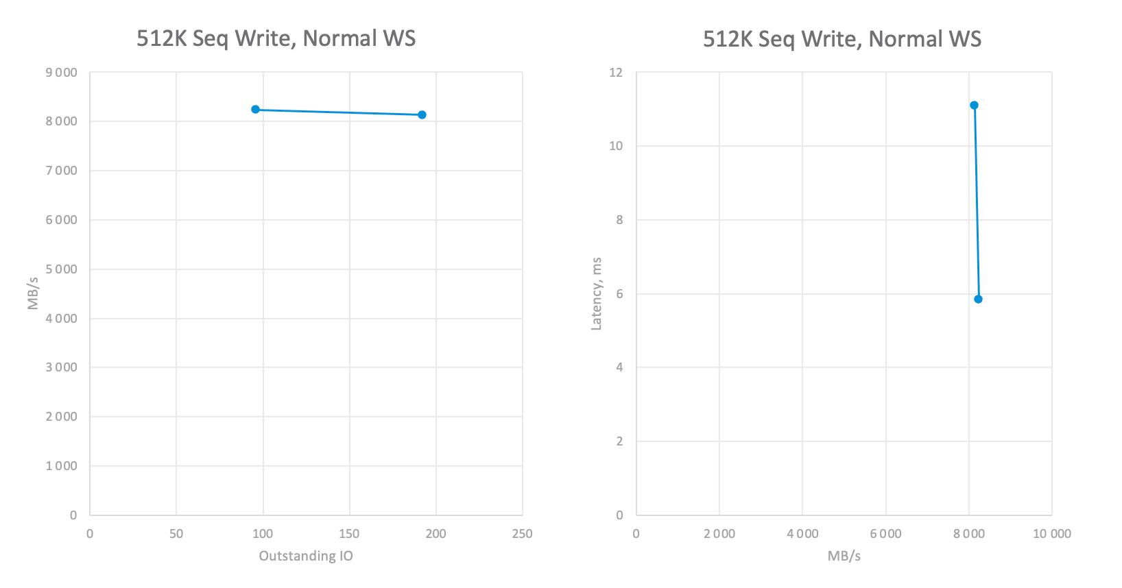
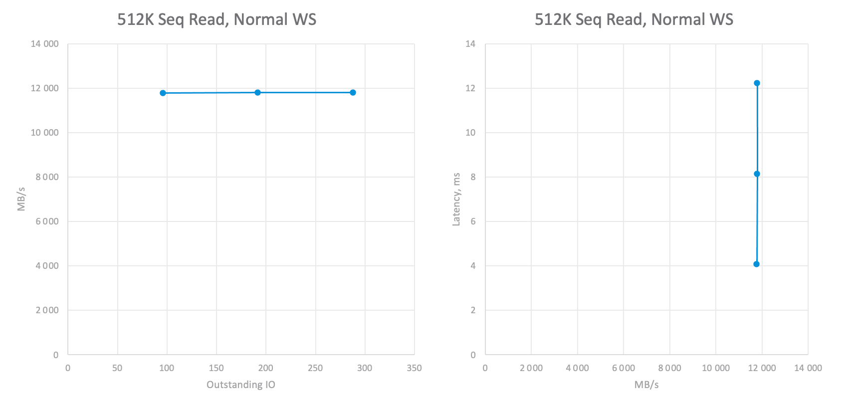
• 512K 100% Read 100% Sequential — workload heavily uses the bandwidth and reveals batch read operations performance. 
• 512K 100% Write 100% Sequential — write-heavy workload, washes out controllers’ write buffers and reveals batch upload operations performance.

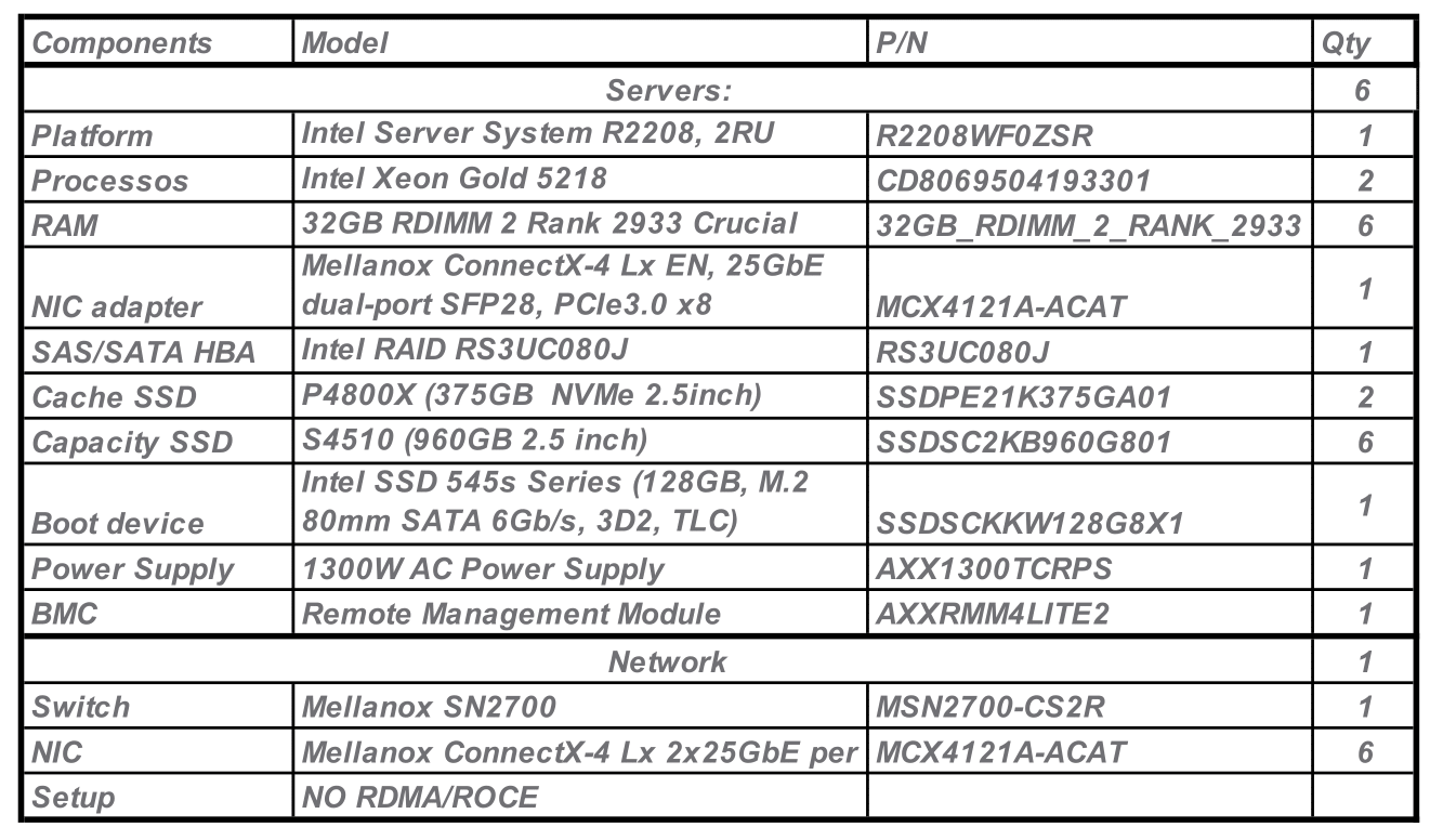
To replicate the scaled-in future production environment, the testbed consisted of 6 all-flash vSAN 7.0U2 nodes." in a configuration almost similar to the target (except for the compute resources).  At the same time, we have evidence that performance scaling occurs linearly, provided that both the number of nodes and the number of VMs increase at the same time. Six nodes are required in order to run tests in various configurations, including tests with the enabled Erasure Coding FTT=2 (aka RAID 6), which requires a minimum of 6 nodes. But for sake of this guide’s conciseness, all tests in this document will refer to the storage policy FTT=1 Mirror (aka RAID1). You can find the detailed configuration of the testbed in Appendix A.

Workers VMs

Based on existing infrastructure’s assessment, about 16 vmdks per host are required. Since the computing resources on each node are quite limited, I decided to place 4 VMs with 4 vmdk on each node. Preliminary tests, as well as observations during the main tests, showed that 4vCPU is enough to avoid a bottleneck.

Further scaling-out the number of VMs or scaling up VMs themselves can only worsen the results due to the high compute oversubscription and CPU resources competition between the VMs.

Size Of the Virtual Disk and the Overall Capacity Utilization.

In the test conditions, it is said that it is necessary to fill the storage to the recommended levels that are used when designing the future infrastructure.

VMware recommends keeping the free capacity of vSAN at about 15–30%, depending on the cluster size and configuration. So, I calculated the size of vmdk to achieve the total capacity utilization of ~75% (~420GB) and this value was taken as a baseline.

Before that, I ran the test with capacity utilization increased from 17% to 98,7% with every workload profile to understand the impact. The most important part here — I did not change the absolute active workload size set in TB during the tests. Also, tests were executed in the steady state (this means data was written and some time passed so no rebalance active operations were running in the cluster). On the graph, the performance at 75% capacity utilization was set as 100%.

We can see that there is no significant performance impact of the higher utilization regardless of the workload profile for the VMware vSAN. The interesting thing found out here is some 7–17% performance degradation at the lowest utilization (17%). The reason for this is because at this level most of the data resides at the write buffer SSDs without destaging to the capacity tier leading to a decreased number of SSDs proceeding the IO requests.

For all next tests 75% capacity utilization will be used.

Active Workload Set Performance Impact Tests

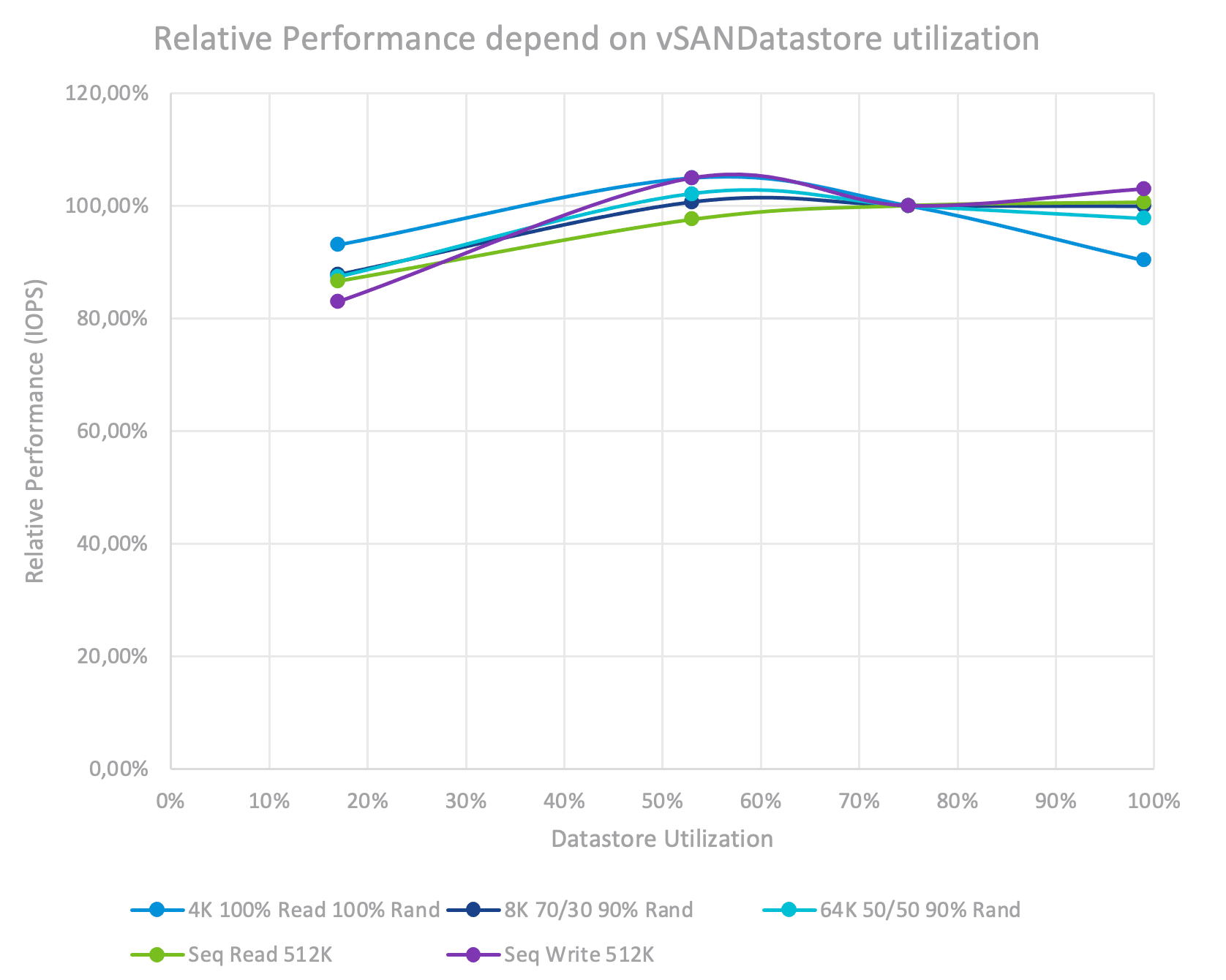
Now let’s investigate how the Workload Set dimensioning affects the performance of the vSAN Cluster. I varied the workload set size from 1% to 100% and measured IOPS and latency for every workload profile.

At 4K 100% Reads we observe almost no impact of the active workload set size. The reason for this is because it was an All-flash vSAN Cluster and it serves reads right from its Capacity Tier without any overhead and SSDs in Capacity Tier can process them really fast. The same picture goes for the sequential read test.

At the same time, it is quite obvious that for a hybrid cluster there would be a very sharp performance drop since running out of the SSD cache.

With the 512K Seq Write test, the picture has dramatically changed. You can see two performance layers — active workload set 1–10% and 30%+. At 1–10% level the system responds at a write buffer speed. We can write data into the write buffer really fast (with the Write Intensive Optane SSD), but once our active data no longer fits into the Write Buffer, the destaging process is triggered. This process affects our front-end performance — vSAN needs to free up some space in the buffer by destaging data to the capacity tier to process new data coming from the worker VM. Beyond 30%+ the destaging becomes continuous and massive, however the system achieves a balanced and steady state.

The mixed workload test is obviously a mix of 100% Read and 100% Write test. Every read is processed fast without any impact, writes are not that massive, hence the destaging process is not so intensive. It impacts the performance but does not limit it. This led to a smoother graph and less performance impact overall.

Conclusions About Workload Set

1. Active Workload Set can always affect the performance. So, you should test it.
2. Performance impact varies with different workload profiles as well as with different storage settings (Deduplication, Compression, Tiering, Caching, etc).
3. Honestly, you should not care much about the exact amount of cache/tier in the storage system in case the cache/capacity ratio is the same as in your target system. Think about it as black-box tests.
4. It is smart to analyze two cases — normal or expected with an active workload set of ~10% (or whatever number you got by assessing your existing environment) and a reasonable worst case of ~30%.
5. Be accurate and change only one variable at a time.
6. Test duration must be sufficient (I will demonstrate this later in the document) to achieve the system’s steady state when caches are warmed up and buffers are full.

For the next tests, I will use 10% WS (“Normal WS”) and 50% WS (“Huge WS”) also for a more holistic view.

Analyzing Test and Warm-up Duration Impact

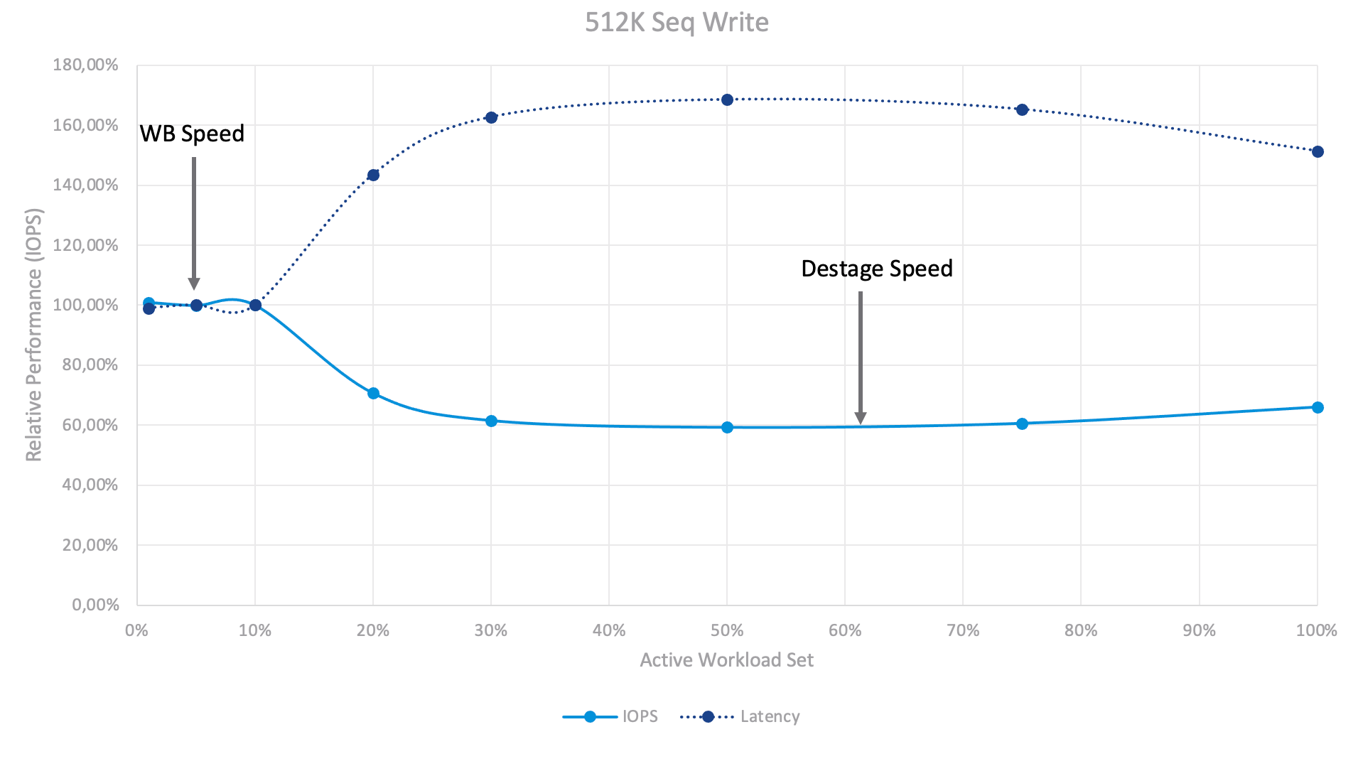
Here are some examples of vSAN cluster performance behavior. For this test I’ve used a “Huge” 50% workload set for better visibility:

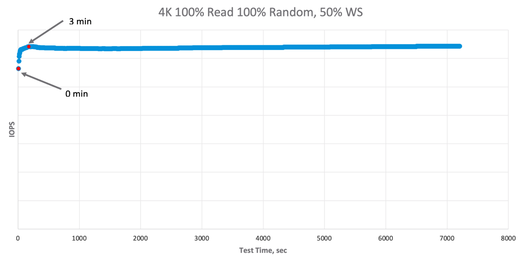
For the reads, we can see that the system achieves a steady state in a few minutes and the difference is quite small. This happens because All-Flash vSAN does not have a sizable read cache (well, technically, it does have a small RAM cache, but it is miniscule compared to the “Huge” workload set of 50%, so the RAM cache hit ratio is close to zero, leading to no-cache warm-up behavior).

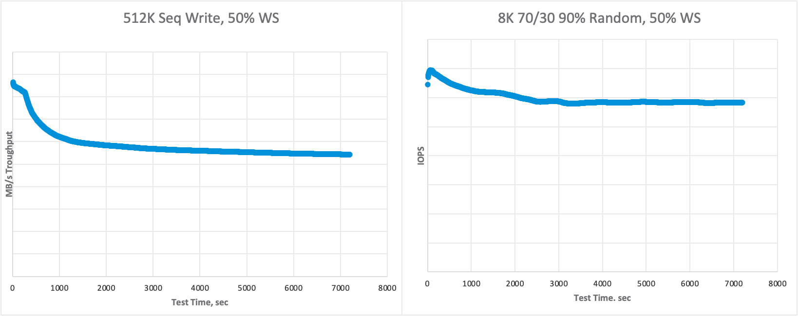
For the writes, the behavior changes dramatically. Because of the write buffer and destaging process, which I explained before, at first, we fill the buffer (and achieve a maximum performance), and, once the buffer is full, vSAN starts destaging. vSAN manages the destaging intensity over time and its performance impact is usually manifested within 1800–3600 seconds (30–60 minutes).

Conclusions About Test and Warm-up Duration

On the one hand, the longer test and warm-up durations provide more confidence over the results quality:

• Impact and volatility vary significantly, depending on the test’s configuration, storage system, its settings, etc.
• The performance difference between the beginning of the test and its end can be significant.
• The longer you test the clearer you see any volatility in the 95/98 percentile.

But if we run each individual test for many hours or days the total time, we need to invest becomes enormous. So, we need to find out the right balance and ways to optimize:

• Look through the data point for the tests to evaluate its steadiness.
• You can significantly decrease the test’s duration in case you are running a set of related tests. For instance, the same workload but with a different number of outstanding IO. The only side effect is — opening tests might not be relevant because of a small warm-up duration, so you should include some “dummy tests” before recording the results.
• You can use shorter tests (like 15-30 minutes) as warm-up pre-runs and, once you understand the needed parameters, you proceed to the final long test and record its result.

The tests in this guide were run with 15 min of warm-up + 30 minutes of test or with 30 minutes of warm-up + 1-hour of test.

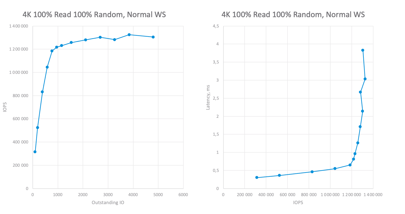
Test the OIO Impact

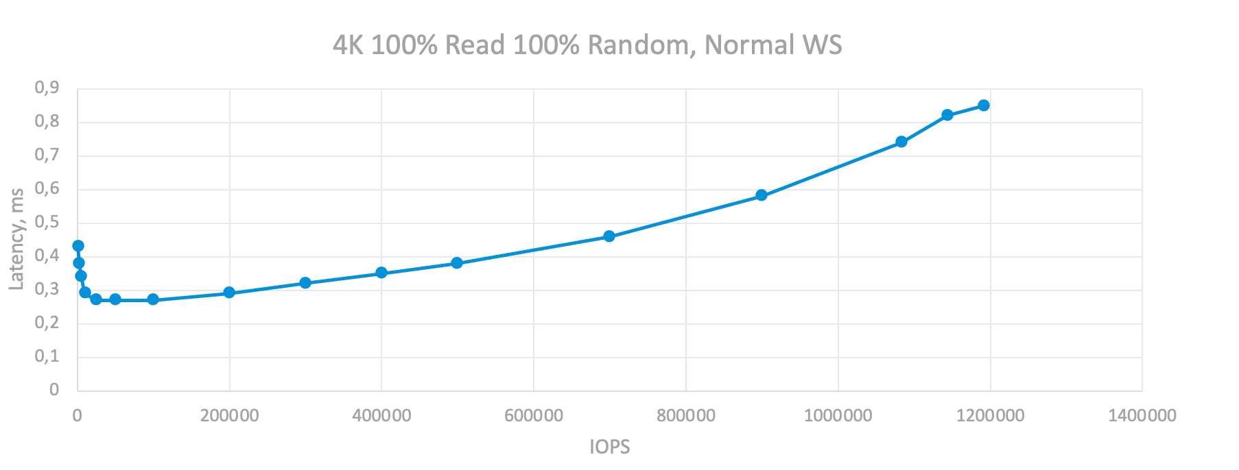
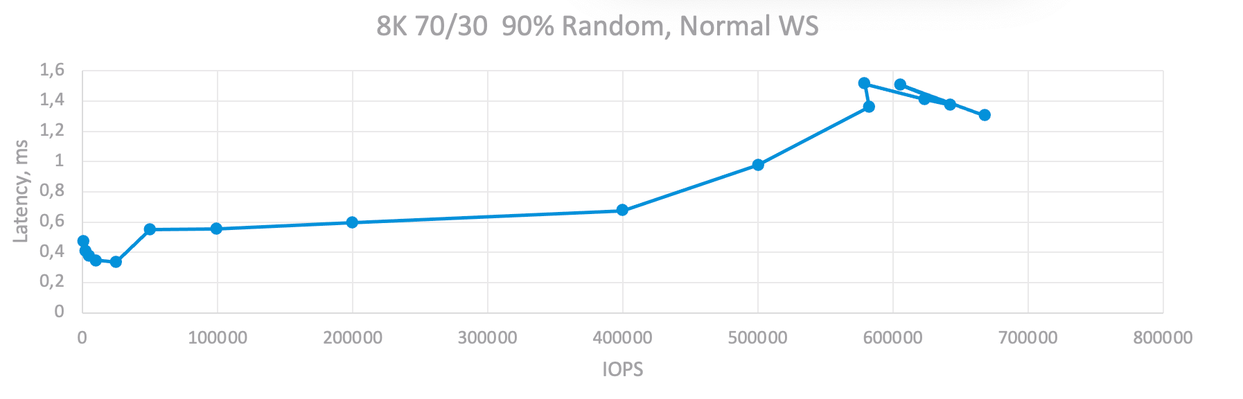
Now we are approaching the main stages of testing, namely, determining the performance of the storage system on the necessary workload profiles. To do this, we run tests at various OIO values, recording performance and latency. As a result, we will get two graphs (in fact, the latency vs IOPS graph is enough for us, but for clarity, I will leave both). Now drawing a line that indicates our latency threshold or adequate maximum if it bellows the threshold and so, we can understand how much IOPS the system can issue under the required conditions:

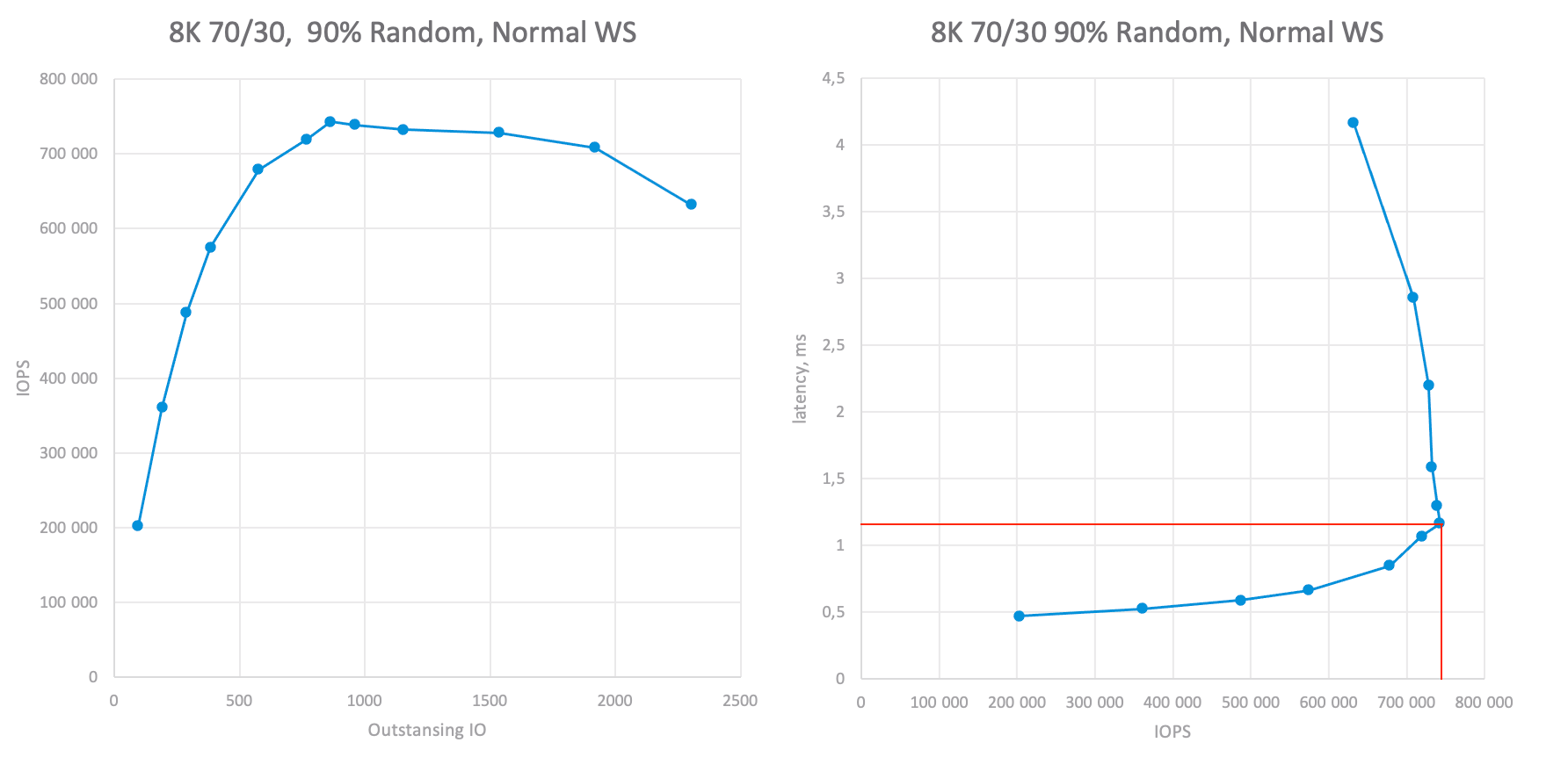
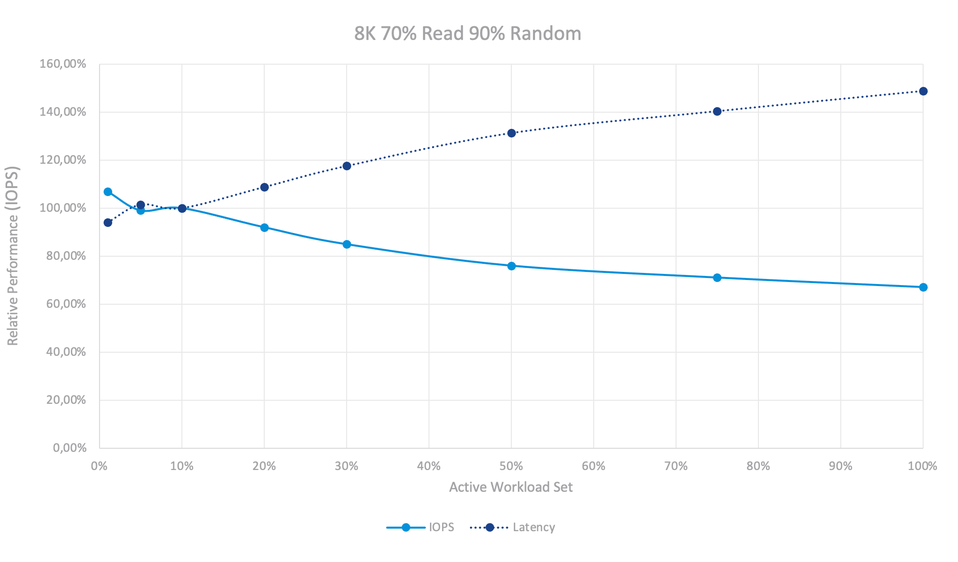
For an 8K 70/30 workload profile six node cluster could achieve ~730K IOPS at ~1.1ms latency. Or 115K IOPS per node which is more than required.

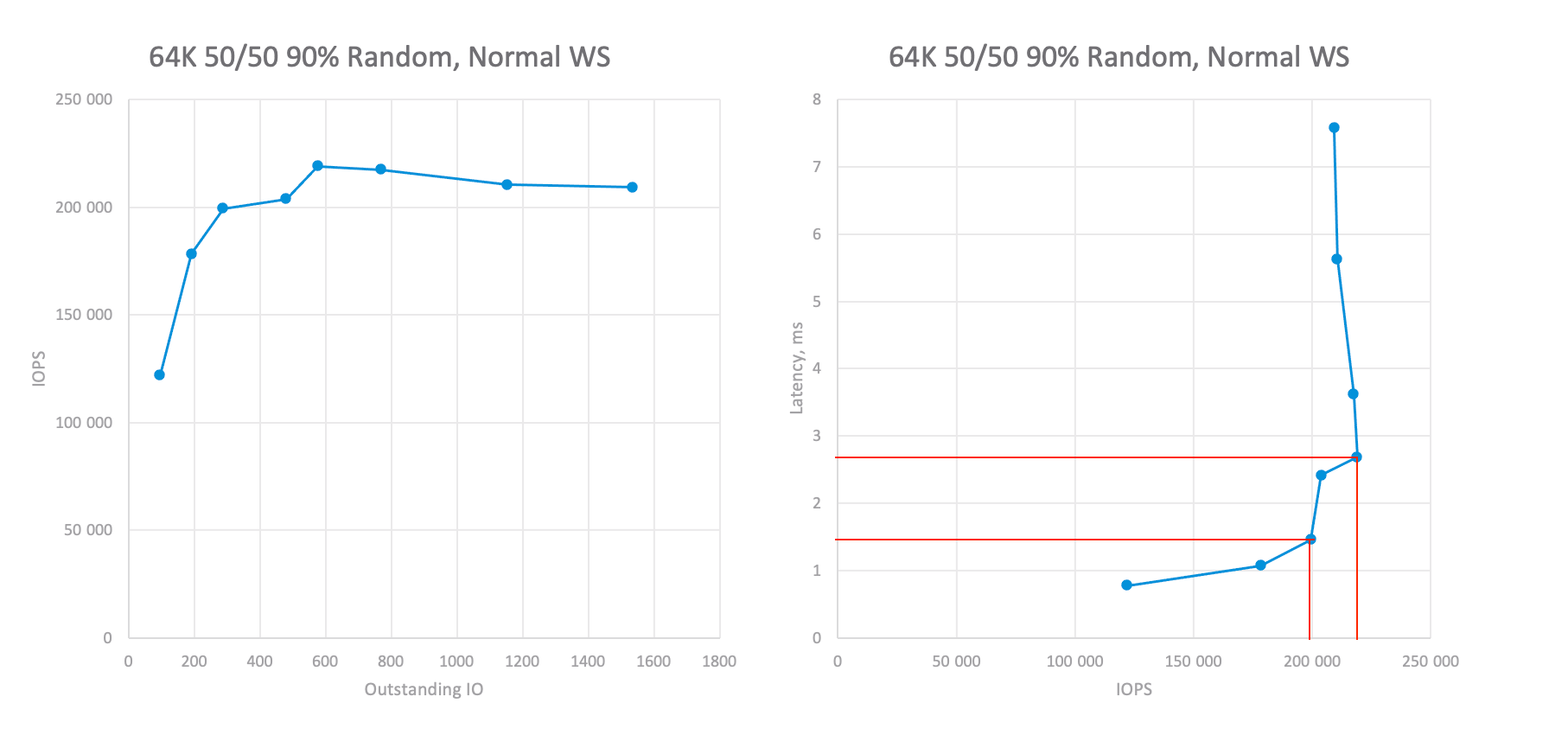
For an 64K 70/30 workload profile six node cluster could achieve ~200K IOPS at ~1.5ms latency and ~220K at 2.8ms. Or ~35K IOPS per node which is also more than required.

Additionally, we will conduct tests for all other workload profiles:

Conclusions about OIO

1. In case you want to understand the storage potential, run the benchmark with different values for OIO to get OIO/IOPS/Latency dependency graphs.
2. From the IOPS/Latency graphs get the value of the maximum IOPS achievable with the latency equal to or below your requirements.
3. You should do this for every workload profile or storage setting because the optimal OIO value will vary.

IOPS Limits.

As an example, I will run tests with the optimal number of OIO, but different values of IOLimit, which will allow me to build a more accurate dependence of the latency vs IOPS and, at the same time, evaluate from almost zero values to the maximum:

Testing Results

Summarizing the intermediate results of the testing, we confirmed the viability of placing the required number of workloads on the vSAN cluster in the planned configuration at normal operational state if RAID 1 storage policy without Space Efficiency is used.

We also learned and understood how each of the parameters can affect the test results, as well as what you should pay attention to and in what cases you can expect an additional drop in performance. Further we do not need to carry out all these tests (such as the utilization, workload set, etc) it will be enough for us to use individual selected parameters.

Now it's worth testing against the required load profiles for other storage policies to determine if they can be used to accommodate different workloads. But I will not include these tests in this guide for the sake of brevity since the method will be exactly the same.

Conclusion.

I hope I was able to show you how the general approaches outlined in the first part can be applied in practice. You could be convinced that by consistently approaching the task, you can relatively easily conduct benchmarking and, most importantly, get a meaningful result.

Also, this material may be of particular interest to those of you who are looking at and planning to use VMware vSAN in their infrastructure. This guide refers to a fairly popular hardware configuration that can be found in a large number of vSAN installations.

Thanks to those who had the time and energy to read such long articles. I invite everyone to the discussion and please share your own experiences and recommendations. So, we can further improve these articles together and bring more value to the IT pros community!

Happy Benchmarking!

Special Thanks.

I would like to express my special thanks to Alexey Darchenkov, Mikhail Mikheev and Artem Geniev for a huge amount of their time, experience, competencies, and invaluable support while creating this guide. Without them it would not have been possible.

I also express my gratitude to Asbis and especially Nikolay Neuchev for providing vSAN demo stand and allowing these tests to be carried out.

Appendix A.

The Hardware BOM:

The software BOM:

• ESXi 7.0 Update 2a (build 17867351) + vCenter 7.0.2.00100 (build 17920168)
• Drivers and Firmware — latest certified from VMware HCL in May 2021
• HCIBench 2.5.3 with FIO

The vSAN settings:

• Storage Policy — FTT-1 Mirror
• RDMA = off
• Adaptive Resync — On
• All other settings are set in the default.