Enterprise Storage Synthetic Benchmarking Guide and Best Practices. Part 2. Success Criteria and Benchmarking Parameters.

Define the Success Criteria for the Synthetic Benchmark.

As I mentioned in the first part of the guide, defining the goals and success criteria is a mandatory step for a successful POC. Of course, success criteria will vary, but they all have something in common — they should follow the S.M.A.R.T. rules:

• Specific — the goal should be specific and clear for everyone involved in testing. There should be no misaligned or ambiguous interpretations or “it goes without saying”.
• Measurable — this means there is a metric or number, which can unequivocally decide pass/not-pass or the result A is better than B.
• Attainable — the requirements should be realistic and achievable (at least in theory) by every participant. Otherwise, there is no reason to spend time on it.
• Relevant — it is the most important item here. You should be able to clarify and very clearly show why such goals and metrics were chosen. How are they linked to the business needs? Why exactly this metric or number and not another? And be careful with references to the “industry standards,” “this is how we did it previously,” “experience in other companies.” It is too easy to make a mistake and lose relevance to your specific business needs.
• Time-bound — your POC plan should have explicitly and upfront defined timelines and deadlines.

The goals, as well as a detailed benchmark program (that describes exactly how the tests will be done), should be written BEFORE the beginning of the POC and approved/confirmed by every participant.

I also recommend sending the draft of the program to the participants, often they can provide some useful advice, recommendations, or comments and in order to get them ready. As well as to be in touch with vendors/partners in the process of the benchmarking especially if there are some issues or the system could not achieve the goals. Often, the issues can be easily solved just with the proper setup and tuning.

A simplified example of the success criteria could look like this: “The latency in guest OSes running on the storage system under normal conditions and fully operational state should be less than 1.5ms at 95th percentile while providing 100K IOPS with profile 8K 70/30 Read/Write 90% Random. The workload is generated by 12 VMs with 5 virtual disks in each, storage utilization (total amount of data stored by these VMs) should be 70% of the useful storage capacity, active workload set size is 10%, test duration 2 hours after 1 hour of the warm-up”.

Initial data and inputs.

The first and the biggest challenge of the benchmarking that appears at the preparation phase is to gather data and the metrics to specify the goals. In the above example there were a lot of numbers, like workload profile, workload sets, required response time, etc. The question is “How, Where, and from Whom can I get all of these numbers?”

In your specific situation, you can explore various ways to collect the data, but the most common are:

1. Get the data directly from the application owners. In theory, they know the best about their app’s requirements. Practically, it is quite rare for the application team to be that much aware and be able to provide infrastructure-related metrics. But at the same time, they have other extremely valuable information - peak periods, components and processes that have a key impact on business users, response time objectives, types of services that run inside the application, etc.
2. Profiling. We can describe the required business services and deconstruct them down to the elements they consist of. Then pick the most critical and/or heavily loaded components and conduct the in-depth analysis of such. We do that by collecting the workload profile stats related to those components. At this point, you should get an accurate application load profile, response time objectives, and an estimate of performance requirements (which can either be equal to the current load or scaled up). This way we can reproduce the workload on the tested system as close as possible. The results will indicate if a particular service is able to run on the tested system or not (from the performance point of view). Having done with one service we will then move to the next one. Just mind the possibility of workload interference if your storage is shared amongst multiple services and explore the options to neutralize or minimize the potential impact in advance.
3. Averaging and generalization. With this approach, we look at the problem from the other side — apps and services are the “black boxes” which create the load onto your storage infrastructure. They show the overall load profile that comes to the storage system from applications as well as current average response time and performance. We can analyze the workload profile and patterns from the storage point of view and try to reproduce the load. Just be aware that it will be harder to notice finer performance issues hidden within this mass, while those can have a significant impact on a particular service.

I recommend combining these approaches for achieving the best results. It makes sense to join forces with app teams to analyze separately the Business-critical apps and services consuming a major part of the storage infrastructure. And augment this analysis with the more generic infrastructure tests if there is a possibility to do so.

Based on my experience, I would recommend the following course of action to you:

1. Define the list of most business-critical workloads, services and apps that are planned to be deployed on the storage system.
2. Have a discussion with the applications’ owners on apps’ components, specifics, key requirements and what you should pay special attention to.
3. Accurately analyze the load profile of these applications in low-level details.
4. Analyze overall metrics from the infrastructure.
5. Create a table showing the workload profile for every business-critical app and for infrastructure overall. 
6. Specify the success criteria for each of them (which usually contain acceptable response time and required performance in IOPS).
7. Agree criteria with application owners and vendors.

Once the workload profile is captured there are several ways to reproduce it. Subject to your goals and objectives, one option is to generate exactly the same amount of load (bandwidth, IOPS with the same block size) and measure the response time to confirm if it is below the required level. This is an effective way for constant and stable infrastructure. Alternatively, you can measure the maximum load that the system can handle. You do so by setting the response time goal and gradually increasing the workload corresponding to the production one till the latency hits the threshold.

Finally, it is also important to analyze a reasonable worst-case scenario. The most obvious example is to test storage in a degraded state. We all know that disks and nodes will fail during the operations, this leads to performance degradation and rebuilds. Another example would be massive trim/unmap requests due to the bulk deletion of data / VMs, or dedup metadata recalculation, or low-level block management, etc. The idea here is to ensure that the system can always provide the required performance, even in the partially degraded or impaired state. But keep it reasonable, in most situations there is little sense in testing the absolutely worst-case scenario, where everything blows-up and all the bad things happen simultaneously (unless it is a mission-critical nuclear reactor safety system or something like this).

Collecting Metrics from Existing Systems.

Ok, so you have chosen the benchmarking approach, and defined which systems and components to analyze. Now you need to collect the data and metrics from these components and infrastructure to create workload profiles, so let’s discuss the popular options. For my example I am going to leverage VMware virtualization platform, however most tools are cross-platform or have an equivalent for other platforms, so the approach will be remarkably similar. I will start from the high-level data and then move to low-level statistics.

First of all, investigate existing monitoring dashboards. Probably there is some amount of required and important data there. Discuss with application owners and infrastructure teams the metrics they pay attention to and that are critical for them. But highly likely, you’ll have to augment that data using additional sources.

Various infrastructure assessment tools can serve as such additional data sources. One of the fastest and easiest assessment tools, wherein providing most of the required metrics is Live Optics. I frequently use Live Optics as it is a free and cross-platform tool. It collects required metrics from 1 to 7 days with absolutely minimal effort to configure. Just download a portable app, run it on any machine that has access to the infrastructure, provide read-only credentials, select the infrastructure segment and analysis’ duration. That’s it. When it is done, you download the report from the cloud portal directly. If your environment is air-gapped and the Live Optics machine has no Internet access, you can manually upload the source data into the portal. The main benefits of Live Optics are ease of use, good enough selection of metrics, including averages and peaks, configurable analysis duration (up to one-week). On the other hand, it is not customizable, and 7 days sometimes are not enough to capture possible spikes or peaks. 

If you need a more flexible tool, you can leverage custom dashboards or reports in your existing monitoring system. It is great if you already have most of the historical values available in your monitoring system, but if not — you can install it fresh and start analyzing the data. One of the commonly used monitoring solutions for VMware Software-Defined Datacenter is vRealize Operations (vRops). It stores most of all required data by default for a long time but lacks out-of-the-box dashboards and reports that immediately fit the storage benchmarking purposes. However, it is not a big deal to create custom dashboards and reports with the required metrics in vRops. You can also create filters for a specific service or a subset of VMs. Just be aware that by default vRops averages metrics’ values collected over 20 seconds intervals into a single five minute data point, so it is sometimes hard to discover short spikes and peaks. This, however, doesn’t create any major challenges for a longer-term analysis.

Ideally, you need both high-resolution metrics (about 20-60 seconds), at least for a few days or weeks, as well as a large amount of historical data, which should take into account periodic peaks (closing quarters, seasonal sales, regular reports, etc.). If it is difficult to obtain both at the same time, then a compromise can be found in the form of metrics of lower resolution (for example, 1-5 minutes), but for an extended period such as a year.

Finally, if averages are not good enough for your purposes, you can use traces. For the VMware platform, there is a great tool called vscsiStats. It is collecting data at the vSCSI device level inside of the ESXi kernel and has a lot of data required for storage profiling. Examples include the distribution of block sizes (not averaged but the actual split), seek distance, outstanding IO, latencies, read/write ratio, and so on. More detailed information can be found in this article Using vscsiStats for Storage Performance Analysis — VMware Technology Network VMTN. For the vscsiStats profiling, you will have to select a VM or VMs and start collecting metrics. By default, vscsiStats collects data points over 30 minutes and saves the data into the file for further analysis. However, keep in mind  that this tool also has some drawbacks that limit its usage - it might itself impact the performance, data collection takes place on each host, vMotion of VMs will hinder data collection and it’s a short-term data collection. 

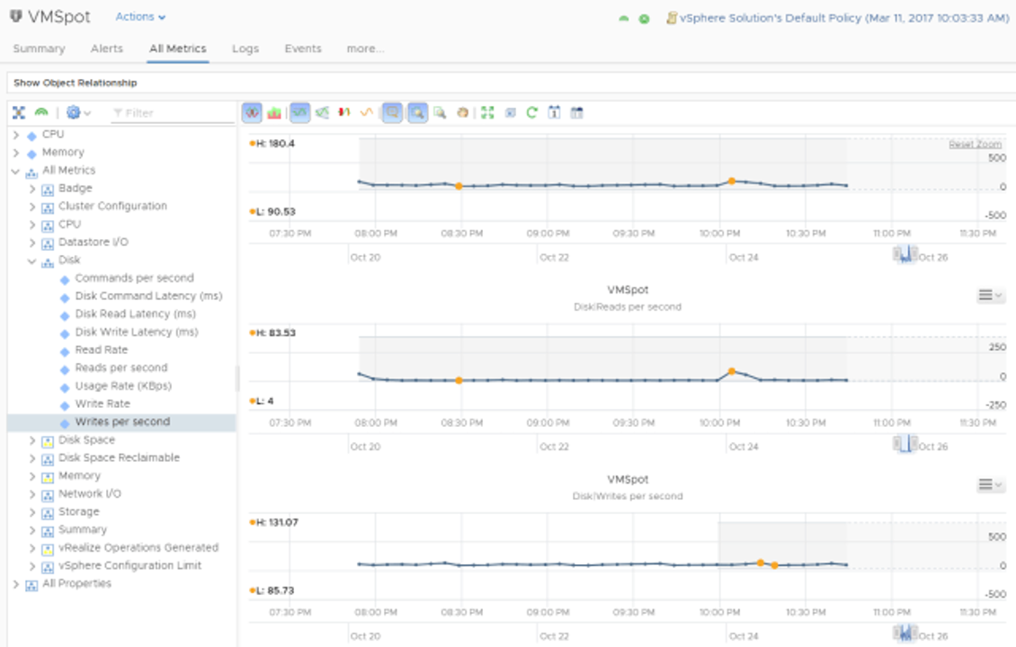
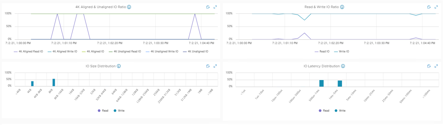
If you are using VMware vSAN there is a tool that simplifies the collection of vscsiStats - vSAN IOInsight. It collects the same metrics and shows the results in vSphere Client, so it is just an easier way to collect traces. There is an example of metrics from vSAN IOInsight:

As an example of a similar tool for the Linux platforms, there is the bpftrace, which can provide the storage metrics at the guest OS level (take a look at bpftrace utilities biolatency, bitesize, and others).

For the most holistic evaluation, you can combine different methods and tools to achieve a comprehensive assessment of the workload. Use the monitoring tool to analyze the long-term performance requirements and identify the most loaded components. And then analyze their workload profiles with vSCSI stats tracing tools.

The List of Parameters to Be Defined.

To run the tests, you must enter several parameters into the benchmarking tool, each of those can have a serious impact on the behavior of the storage system. 

The main principle of the valid synthetic benchmarking — EVERY variable/parameter/number:

1. Must be explained and understood, there must be a clear understanding why exactly this number is chosen.
2. Must be written and documented.
3. Must be agreed with every POC participant.

The easiest way to self-check is to ask yourself: “Why did I choose this number and not another?”. If the answer is “I took this number from the assessment of the existing infrastructure” or “This is the requirement from the business/application owners” or “This is a recommendation from Best Practice and it's suitable for our future use” then it’s ok. If there is no answer or “some guy on the Internet told me it’s right” or “I saw this number in someone else’s benchmark” please pause and re-consider. Think about what this parameter really means and how you can define its value.

Let’s define the list of the general variables you should define based on the HCIBench example:

1. Workload profile:
1. Block Size
2. Read/Write Ratio
3. Random/Sequential Ratio
2. A number of workers VMs and their configuration.
3. Size of the virtual disks
4. Active Working Set
5. Test duration and Warm-Up Time
6. Number of Threads/Outstanding IO
7. IO Limit

Let's go one by one explaining what they mean and how to define them. 

Workload profile

Workload profile defines the specific pattern(s) of IO requests sent to the storage system. It has the following dimensions:

• Block size. It is the size (typically in KB or MB) of read and/or write request sent from Guest OS/Application to the storage.
• Read/Write Ratio. It is the ratio of read operations to write operations.
• Random/Sequential Ratio. Sequential IO is a sequence of requests accessing data blocks that are adjacent to each other. On the contrary, Random IOs are requests to unrelated blocks each time (with greater distance between them). Good illustration is here.

Every tool for collecting metrics I’ve described above, will provide you an average block size and read/write ratio. So, you just need to investigate it and you will get average numbers outlining your infrastructure.

It is a bit harder to assess the requests’ “randomness,” since this requires tracking LBA addresses of every request to determine seek distance. And it’s possible only with tracing tools like vSCSI stats or bpftrace. However, if you are running a virtualized or mixed environment, the IO requests will be of mostly random nature (exceptions to this rule include backup jobs, copy, upload operations and so on, but they rarely directly affect business processes). Hence, for such environments it makes a lot of sense to run most of the tests at 90-100% of Random IOs.

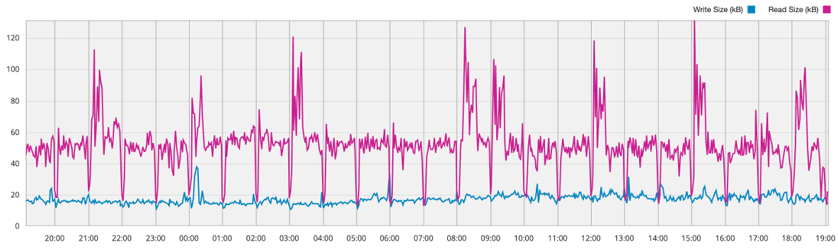
Most often averaged numbers are used to describe the workload profile. However, I strongly recommend analyzing and reproducing the exact block size distributions. Because in real life it’s always a non-uniform mix of blocks with different sizes. Here is just an IO pattern example, captured with vscsiStats for a real-world application:

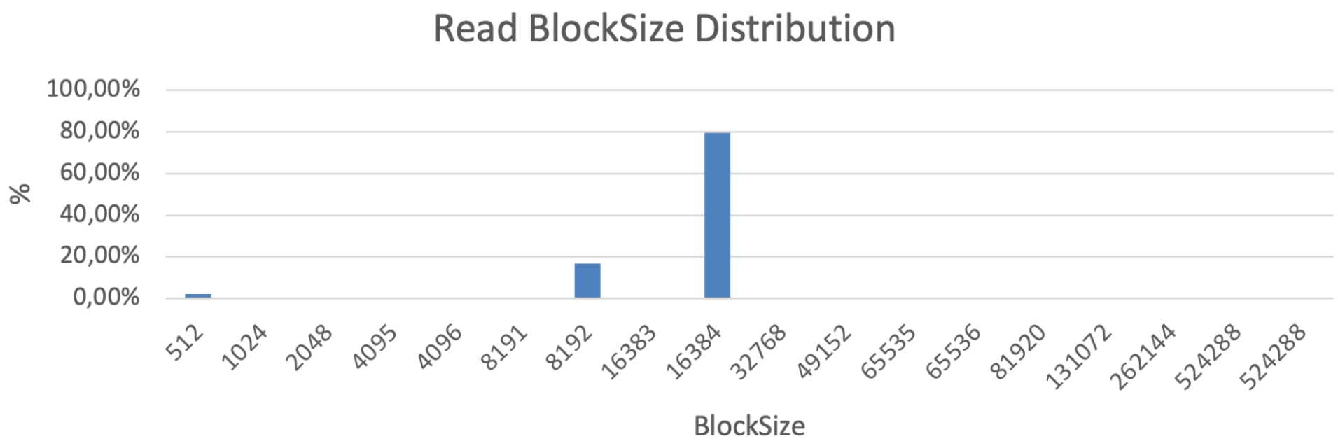
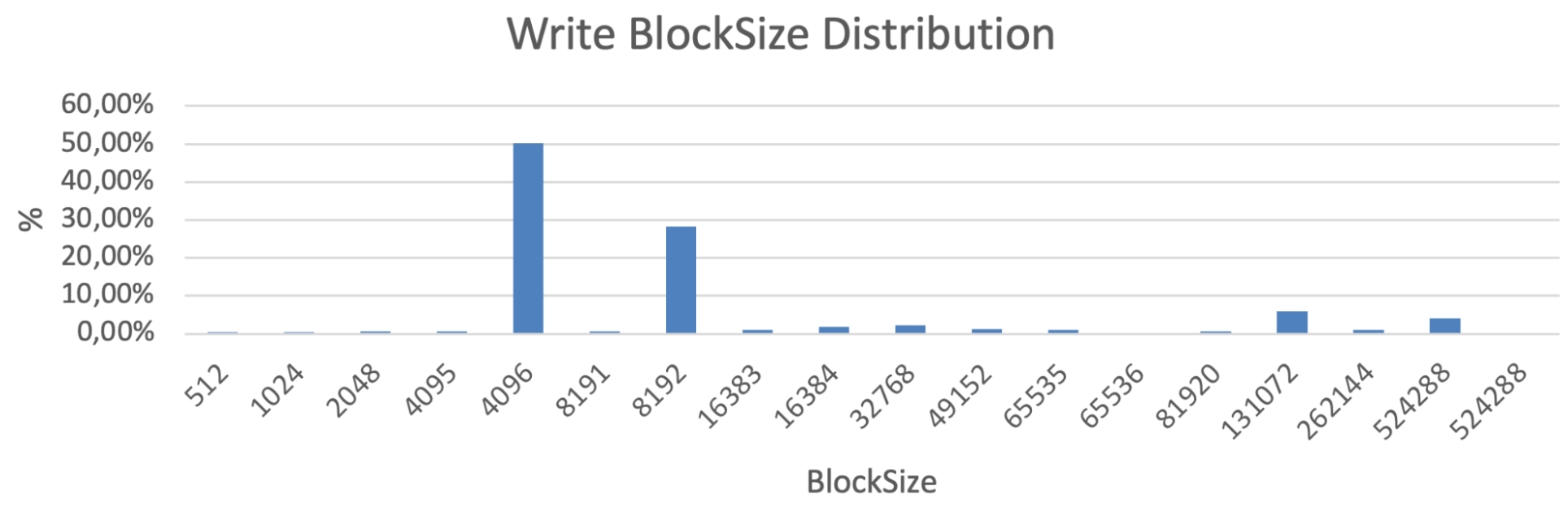
In this example, most blocks are 8K and 16K for Reads, and most of the writes are 4K and 8K, but there are also some ~128K and 512K blocks. And this small number of huge blocks can make a significant difference, because they are filling up the storage write buffers and consume the bandwidth thus preventing the fast processing of small blocks. Therefore, even though the most popular write block size is 4-8K in this case, and the average is ~ 30KB, it is incorrect to run a benchmark with 30K blocks, and even more so 4-8K blocks.

Worker VMs

You also should define the number of worker VMs and their configurations, especially the number of virtual disks, number of vCPU, and vRAM amount per worker.

The choice of vCPU and vRAM per worker is quite straightforward. The idea is to avoid the bottlenecks within the workers themselves and at the virtualization platform level, thus making sure that the benchmarking results are isolated to the storage system only. So, you should just verify there is no 90–100% CPU utilization inside the workers and the platform. In ordinary cases (when it is not one worker rushing the whole storage but a lot of them), 4 vCPU/8GB RAM or 8vCPU/16GB RAM are ok. The most indicative test to check for the reasonable CPU utilization is 4K 100% Read. Immediately after the deployment, you can run this test to verify that you have not hit the compute limits. But even after, you should periodically check the utilization during the tests.

The number of VMs and the number of virtual disks (vmdks) is a little bit more complex. You should analyze the rough ratio of the vmdks per host in your environment and replicate it as much as possible during the benchmarking. By placing multiple vmdks we are avoiding the potential bottleneck with the vSCSI adapter and balancing the load. While using only one vmdk per worker VM can dramatically increase the number VMs leading to high vCPU oversubscription ratios and hiding the true storage system performance behind the stressed platform. This may be a challenge when your physical hosts resources are lacking. That said, it makes sense to use several vmdks per worker VM. A typical number of workers is 2–8 VMs per host and 2–10 vmdks per VM (which closes most cases in the range of 4-80 vmdks per host), but it is always better to validate the numbers yourself in your own environment. 

Size Of the Virtual Disk and the Overall Capacity Utilization.

The size of the vmdk defines how much data you STORE. Total capacity is defined as the number of VMs multiplied by the number of vmdks per VM multiplied by the size of each vmdk. It has nothing to do with the data access. For example, it could be a cold archive — write once - read almost never, but you still store it. How to define the total capacity required? In case you have a scaled-down system for the test it should be defined as the percentage of the total capacity. This number should be aligned with your future storage environment. For example, if you need to store 100TB of usable capacity and the storage system vendor recommends you not to exceed 80% utilization because of the performance impact, you need to purchase 125TB of usable capacity (after raid/spares/system/etc). So, if a vendor provides you a 50TB system for a test, you should fill it at an 80% level by uploading 40TB of data.

Also, the critical part is to enable the PREPARATION of this capacity. This means you need to write down the whole amount of data before starting any test. I always recommend running the preparation with random data, not zeros to avoid undesirable specific behavior storage might have for the processing of bulk zeros (e.g. deduplication, compression, or zero-detection).

It is quite interesting to analyze the impact of high-capacity utilization, especially when you are evaluating the worst-case scenarios too. In some storage systems, a high-capacity utilization can dramatically impact the performance due to internal processes. And the unexpected storage space overconsumption can happen due to an operator’s mistake or poor planning or other unforeseen circumstances. Thus, it makes sense to test not only with the planned/expected utilization but also with the higher numbers to understand the behavior, risks, and the potential impact.

Active Workload Set

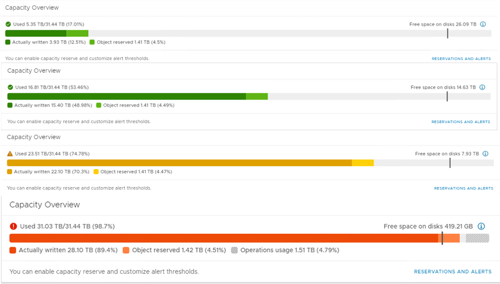
Active Workload Set or just Workload Set (WS) sometimes confuses people. To make it clear — it is an amount of data you ACCESS or in other words actively working with. This heatmap is good example to illustrate an active workload set vs the total capacity:

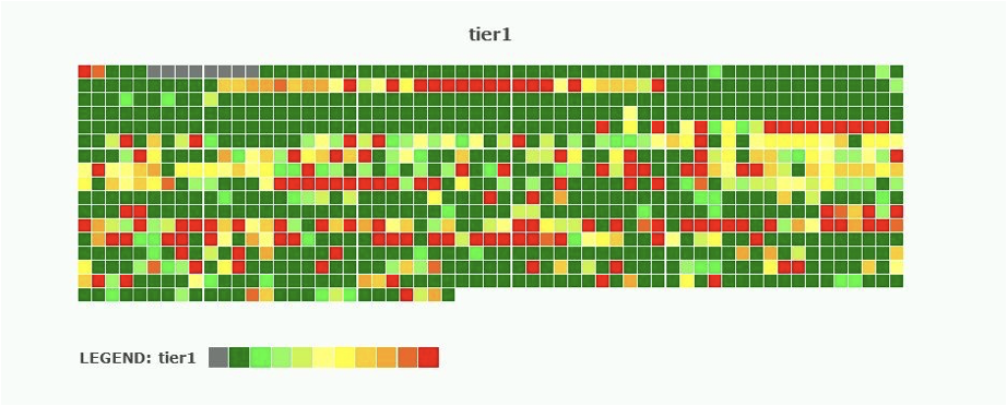
Here the total amount of bricks illustrates the amount of data you store, and their color indicates the amount of data you actively work with. For example, if you evenly process every GB you have written, the active workload set will be equal to the total capacity and every brick should be marked in red.

In fact, this almost never happens. Even if most of the data is analyzed it is not done at the same time — one day we are working with one block of the data and with another the next day. Also, most of the data is rarely touched at all. Just imagine the system disk of any OS — most of the data, files, and packets are used extremely rarely, wherein others are processed at every reboot.

The problem is how to analyze the amount of active workload set as the percentage of the usable capacity. And it is one of the most challenging metrics to analyze in your existing infrastructure. Some options we have:

1. Daily Writes in TB. It is quite easy to acquire (Write Performance in MB/s multiplied by the duration of the writes or more strictly speaking it’s an integral of the write throughput over the time). The problem here is that we can’t separate “net new writes” and “existing records re-writes”. For example, if an application constantly rewrites 10GB in the loop for an entire day, we will see a lot of daily writes, but the true active workload set is only 10GB. The second issue — it does not account reads, and the amount of data read. But still, it is the easiest way to somehow evaluate the active workload set.
2. The second option is to analyze the size of the incremental backup. It is also easy to do (Of course you make backups, right?) and provides the real amount of data changed. But still, no accountability for reads.
3. The third way is to examine your existing storage system. Almost every storage has a write buffer and a read cache. You know the size of both and by looking into the destaging activity (data eviction from the write buffer to the next tier), read cache miss ratio as well as how full they are you can more or less accurately estimate the active workload size.

Speaking about averages and industry guidelines (Yes, I remember that I asked not to rely on “industry averages,” but sometimes it is really hard to avoid this), you will see quite close estimates — the workload set is 5–15% of the total capacity. VMware points to ~10%. In case you want to test the worst-case scenario, 30% is a reasonable number that well overlaps the regular ~10%.

Test and Warm-Up Durations.

During the tests there are processes that lead to performance variations. Most of them are caused by the effect of various buffers, caches, and tiers. Because enterprise workloads generate continuous load to the storage system it is important to measure not the transient but the steady-state performance.

Warm-up helps eliminate initial transitional processes and to enter a steady state. It is just a period of time when workers process the requested workload, but the results are not captured. The warm-up duration should not be less than it takes for the transitional processes to settle down.

The duration of the test should be sufficient to analyze the behavior of the storage system in the long run. It is important to measure how consistent the results are and, in particular, the response time. Steady-state response time is a critical metric. Imagine, that your app is enjoying 1ms response time for the first 30 minutes, and for the next 5 minutes it goes up to 30ms to return back to 1ms once the buffers are flushed. The average latency will be ok, but these spikes should be discovered. Thus, it makes sense to measure not only the average latency but also its percentile (there is a great post about it from Dynatrace Why averages suck and percentiles are great | Dynatrace news). You can pick your own percentile to measure, but the most common are90th, 95th, or 98th. The higher percentile you set, the more stable and constant latency you will get. On the other hand, with the higher percentile value, you risk missing the transitions’ impact and, potentially, get a more littered result.

So how to understand what will be sufficient warmup and test durations? Look at the data points in the FIO/vdbench report. They not only show the final results but can also record the intermediate values during the test. Look into it and if you notice a significant difference over the test duration, then the tests are not performed in a steady-state, and you should increase the warm-up duration. Test duration can be set twice as long as the warm-up duration to be sure that you catch the impact of any extra internal operations of the storage system you test. Most likely, if the initial transitional processes take X time to settle down once the tests start, those extra internal processes should reveal their impact earlier on the loaded system.

Outstanding IO or iodepth (OIO).

Outstanding IO (OIO) or iodepth indicates in a nutshell the degree of parallelism. The more OIO are configured the more requests will be sent to the storage system from workers in parallel.

If you run validation tests with a number of IOPS equal to your production workload, you can simply configure the same total OIO from the workers. But if you want to uncover the full potential of the storage system you must vary the OIO to find out the point of best performance.

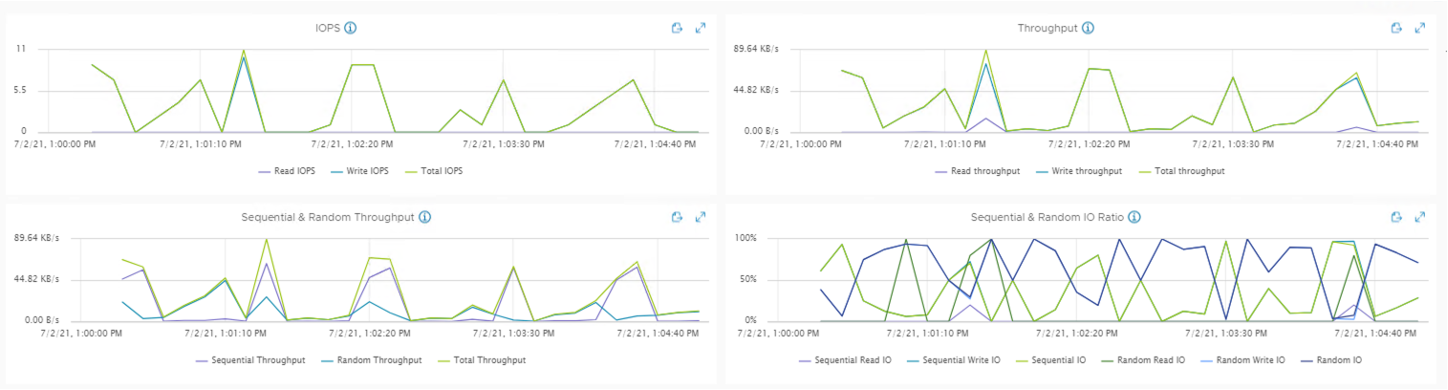
It is imperative to understand that storage is a reactive system. It does not generate anything itself, it only responds to the request from its clients. This is why there may be situations where clients generate a little load easily handled by the storage system. Storage is underutilized and has an enormous potential, but to demonstrate its potential we need to increase the load and the number of requests. Or, alternatively, the storage system may be fully utilized and cannot provide more IOPS. In this case, should you increase the number of requests, you will observe higher latencies, but not an increase in IOPS. And only somewhere in the middle, there is a balanced trade-off of latency vs IOPS in the operating mode. Hence, the dependency between IOPS and OIO from the latency perspective manifests itself like on the below graph:

Therefore, you should vary OIO to obtain the “optimal” number of OIO. What is “Optimal''? It is the amount of OIO where the system provides maximum performance (IOPS) while latency is equal to or below your required level. The challenge is that this “optimal OIO'' will be different for different workload profiles, system settings, etc. This means that every test should be run not at a single OIO setting but with multiple OIO values in the neighborhood of the “optimal point.” Thus, you will ensure that you’ve discovered the correct OIO value.

To do this, run tests starting at low values and gradually increase them. By analyzing the results, you can determine what mode the storage system is currently in. Thus, if you see a significant increase in performance at about the same latency, then you should specify even higher values ​​of OIO. And vice versa, if the delays increase sharply, and the performance practically does not change, then reduce the values of OIO. Do this until you get a few results in the normal mode in the vicinity of the latency threshold.

You will end up with two graphs IOPS/OIO and IOPS/Latency. After that, just cut off its upper at your required latency value and you will get your “optimal OIO'' as well as “Max IOPS.”

IOPS Limits.

Additionally, if you need more precise IOPS/Latency dependency graphs, especially on the wider range of values, you can run the benchmark with IOPS limits set. The pointhere is not to change the parallelism, but the request rate with the optimal outstanding OIO.

To do so, after defining the optimal OIO you run multiple tests with different IOPS Limits from small one to unlimited. Be aware that starting from some value of IOPS limits, the dots (IOPS and latency) will start to converge and match. This is ok because this means that you’ve hit the IOPS maximum and no matter what limit you set you get the same result.

Conclusion.

In order to conduct a successful benchmark, move consistently and do not skip any of the steps - from defining a goal to describing methods and approaches, and then to specific parameters and conditions for conducting tests.

And remember that one of the key indicators of quality testing is the presence of a clear description of ANY parameter used in the test, as well as the presence of an explanation of how it links to tasks and goals.

If you follow the general principles described in this document and adapt them to your situation, then you can be certain of the results and conclusions’ quality.

And now let's move on to a specific example in Part 3, where most of the points previously described in this document will be considered in practice.